Asymmetry curve based on depths

Produces an asymmetry curve estimated from given data.

asymmetryCurve(
  x,
  y = NULL,
  alpha = seq(0, 1, 0.01),
  movingmedian = FALSE,
  name = "X",
  name_y = "Y",
  depth_params = list(method = "Projection")
)

Arguments

x	The data as a matrix or data frame. If it is a matrix or data frame, then each row is viewed as one multivariate observation.
y	Additional matrix of multivariate data.
alpha	An ordered vector containing indices of central regins used for asymmetry curve calculation.
movingmedian	Logical. For default FALSE only one depth median is used to compute asymmetry norm. If TRUE --- for every central area, a new depth median will be used --- this approach needs much more time.
name	Name of set X --- used in plot legend
name_y	Name of set Y --- used in plot legend
depth_params	list of parameters for function depth (method, threads, ndir, la, lb, pdim, mean, cov, exact).
method	Character string which determines the depth function used. The method can be "Projection" (the default), "Mahalanobis", "Euclidean", "Tukey" or "LP". For details see depth.

Details

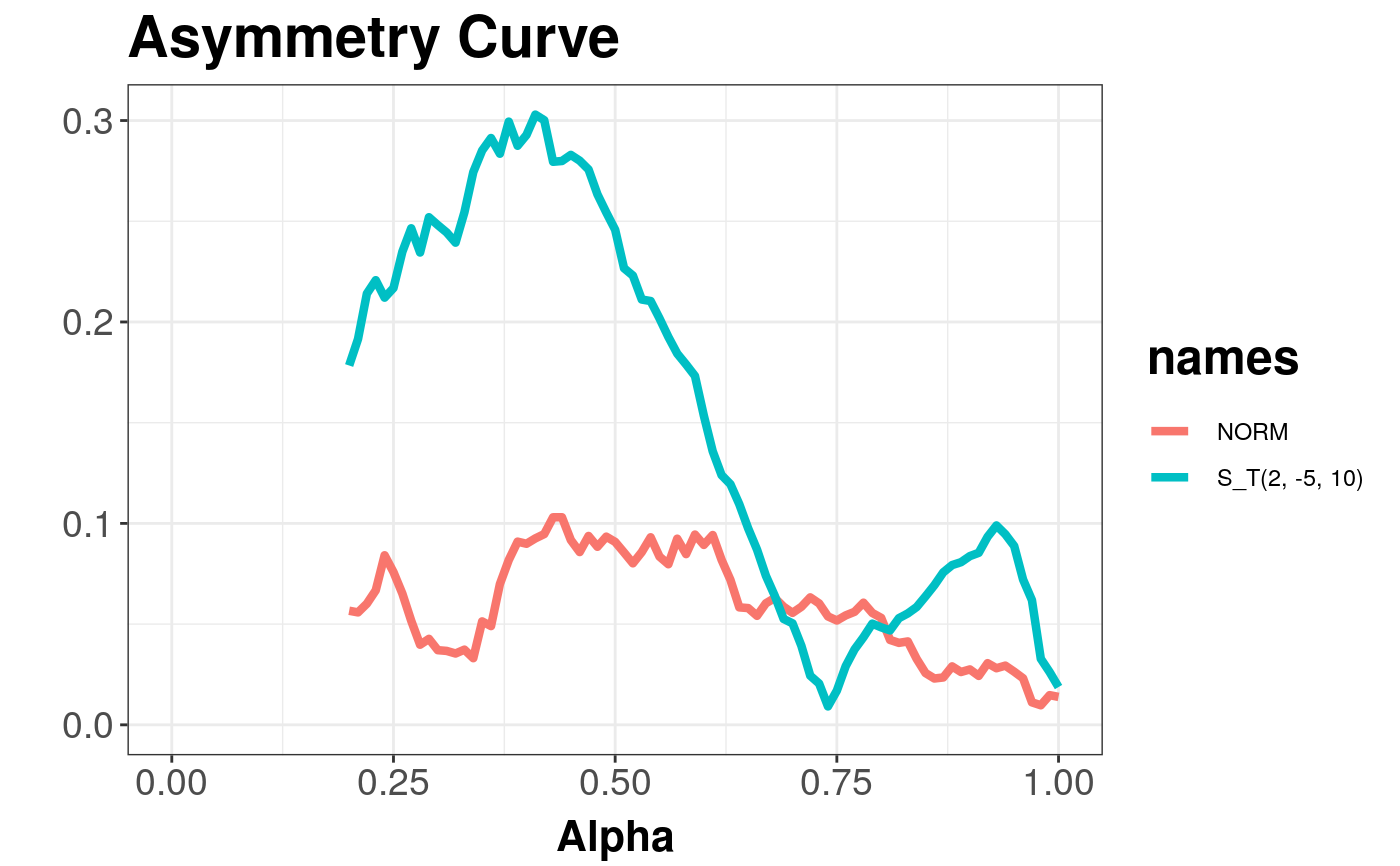
For sample depth function \( D({x}, {{{Z}} ^ {n}}) \), \( {x} \in {{{R}} ^ {d}} \), \( d \ge 2 \), \( {Z} ^ {n} = \{{{{z}}_{1}}, ..., {{{z}}_{n}}\} \subset {{{R}} ^ {d}} \), \( {{D}_{\alpha}}({{{Z}} ^ {n}}) \) denoting \( \alpha \) --- central region, we can define the asymmetry curve \( AC(\alpha) = \left(\alpha, \left\| {{c} ^ {-1}}(\{{\bar{z}} - med|{{D}_{\alpha}}({{{Z}} ^ {n}})\}) \right\|\right) \subset {{{R}} ^ {2}} \), for \( \alpha \in [0, 1] \) being nonparametric scale and asymmetry functional correspondingly, where \( c \) --- denotes constant, \( {\bar{z}} \) --- denotes mean vector, denotes multivariate median induced by depth function and \( vol \) --- denotes a volume.

Asymmetry curve takes uses function convhulln from package geometry for computing a volume of convex hull containing central region.

References

Serfling R. J. Multivariate Symmetry and Asymmetry, Encyclopedia of Statistical Science, S Kotz, C.B. Read, N. Balakrishnan, B. Vidakovic (eds), 2nd, ed., John Wiley.

Liu, R.Y., Parelius, J.M. and Singh, K. (1999), Multivariate analysis by data depth: Descriptive statistics, graphics and inference (with discussion), Ann. Statist., 27, 783--858.

Chaudhuri, P. (1996), On a Geometric Notion of Quantiles for Multivariate Data, Journal of the American Statistical Association, 862--872.

Dyckerhoff, R. (2004), Data Depths Satisfying the Projection Property, Allgemeines Statistisches Archiv., 88, 163--190.

See also

scaleCurve, depth

Examples

# EXAMPLE 1
library(sn)
#> Loading required package: stats4
#> 
#> Attaching package: ‘sn’
#> The following object is masked from ‘package:stats’:
#> 
#>     sd
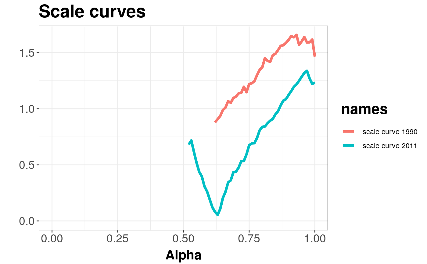
xi <- c(0, 0)
alpha <- c(2, -5)
Omega <- diag(2) * 5

n <- 500
X <- mvrnorm(n, xi, Omega) # normal distribution
Y <- rmst(n, xi, Omega, alpha, nu = 1)
asymmetryCurve(X, Y, name = "NORM", name_y = "S_T(2, -5, 10)")
#> Object of class: AsymmetryCurveList
#> Warning: Removed 40 rows containing missing values (geom_path).

# EXAMPLE 2
data(under5.mort)
data(inf.mort)
data(maesles.imm)
data1990 <- cbind(under5.mort[, 1], inf.mort[, 1], maesles.imm[, 1])
data2011 <- cbind(under5.mort[, 22], inf.mort[, 22], maesles.imm[, 22])
as1990 <- asymmetryCurve(data1990, name = "scale curve 1990")
as2011 <- asymmetryCurve(data2011, name = "scale curve 2011")
figure <- getPlot(combineDepthCurves(as1990, as2011)) +
  ggtitle("Scale curves")
figure
#> Warning: Removed 114 rows containing missing values (geom_path).